
How Ridge or Bayesian machine learning libraries can improve proxy accuracy and robustness.
Foreign exchange (FX) risk generated in first-world countries is readily managed by tapping into the deep and liquid hedging options that are available. However, organizations doing business in emerging markets—whether companies, charities, or investment funds—face a significant and double-edged challenge. First, emerging-market currencies are typically more volatile than major currencies. And second, hedging instruments may not exist for these currencies. Where hedging instruments do exist, they are often prohibitively expensive, due to forward points.
If an organization needs to manage FX risk for an emerging-market currency, the only choice may be to use a proxy. Proxy hedging is not uncommon. One good example is the way that airlines hedge jet fuel using heating oil futures. Fuel costs account for about 25 percent of airlines’ operating costs, and price variation has a large effect on profitability, so hedging fuel costs can be very helpful. Until recently, there were no futures contracts for jet fuel. However, because fuel oil prices closely track (for the most part!) with jet fuel prices, fuel oil futures form a reasonable proxy hedge.
FX risk managers have used proxy hedging for years, too. Before the advent of the euro, companies and traders with exposure to the illiquid Swiss franc (SFr) often hedged that exposure with the more liquid Deutschmark. The use of a proxy currency to hedge FX risk mimics a non-deliverable forward contract (NDF). For example, a UK-based treasurer with exposure to the SFr might have executed a hedge denominated in Deutschmarks. At the end of the hedge tenor, he would still exchange SFr for GBP; the hedge gain/loss would be similar to a direct hedge gain/loss.
The biggest challenge—and the key to successful risk management—is to find a proxy with a strong correlation to the target asset. If the proxy moves in the opposite direction from the hedged currency, or (more likely) moves in the same direction but at a significantly faster or slower rate, then obviously the proxy is not effectively mitigating the organization’s risk. Poor correlation leads to high portfolio variance.
When hedging emerging-market currencies, corporate treasurers may find that it is very difficult to identify a single proxy currency with a useful level of correlation. In such a circumstance, companies can harness statistical analysis and new machine learning technologies to develop a more effective hedge.
Overview of the Basket Approach
One way to improve correlation between a currency and its hedge is to use a “basket” of three to four proxy currencies, each of which contributes a fraction of the hedge. For example, movement of the Chilean peso vs. the U.S. dollar (USD-CLP) might be hedged using a basket of forwards denominated in New Zealand dollars (USD-NZD), Canadian dollars (USD-CAD), and Australian dollars (USD-AUD). Such an approach, in essence, creates a synthetic NDF.
A corporate treasurer considering this approach could use linear regression to determine the optimum fraction of the basket to allocate to each proxy currency. The inputs into the regression analysis would be the historical movement of all the selected currencies. The output would be the ideal weight within the basket for each currency. The goal would be to ensure that the correlation between movement of the target asset (the actual currency to which the organization has exposure) and the proxy basket remains high over a wide range of values for the target asset.
Before getting into the weeds of the decisions around choosing a proxy currency basket, it may be helpful to visualize the basic process for a regression analysis. Regression analysis is a process for quantifying the relationship between variables. The relationship may be modeled using different models—the simplest being a linear model. For the series of data in Figure 1, we can calculate the best fit line (a linear model, Y = aX + b) to arrive at Y = 2.14X + 5.4.
Figure 1
Calculating the Best Fit Line with a Linear Regression Analysis
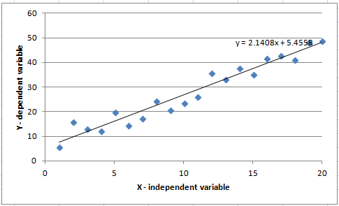
The method for calculating the best fit is called “least squares”; the goal is to minimize the sum of the distances between the discrete data points and the model.
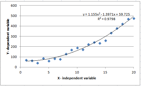
For more complicated relationships, a polynomial of higher order may fit best. Figure 2 illustrates a second-order fit (i.e., Y = aX^2 + bX + C). Note the R2 term: This represents the accuracy of the fit. The closer to 1.0, the more accurate the fit.
Figure 2
Calculating Best Fit with a Polynomial Regression Analysis
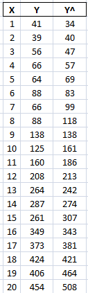
Introducing our notational conventions, table 1 shows X (independent variable), Y (measured dependent variable), and Y^, the value determined from the regression equation we've determined.
Table 1
One more fundamental concept is multivariate regression. The two examples above calculate Y as a function of X. The concept can be extended to functions of multiple variables (e.g., F = aX + bY + cZ.) Regression in this case would quantify all three coefficients—a, b, and c—for the best fit.
Figure 3, below, represents the matrix of inputs into a regression analysis. Each column in the matrix (X) represents a particular currency in the proxy basket—NZD, CAD, and AUD in our example. Each row in the matrix represents a date. Each cell, therefore, houses the value of one currency on a specific date. Separately, column Y represents the value of the target asset—CLP in this case—on each of the same dates.
Figure 3
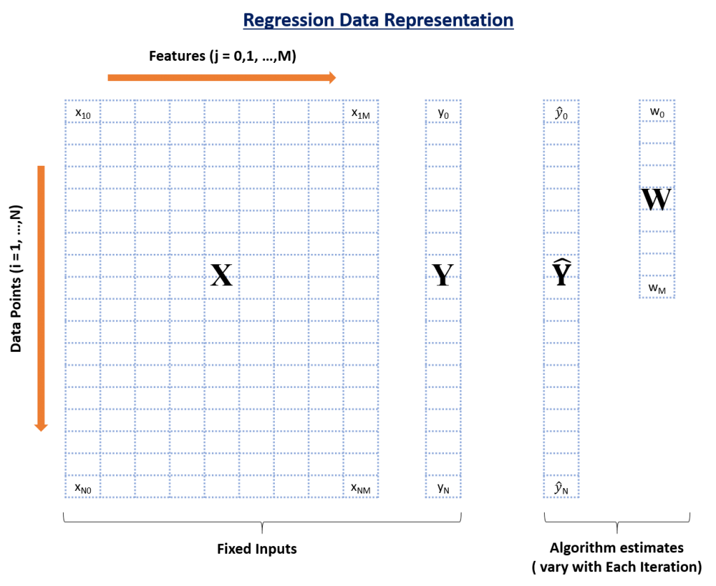
When the regression analysis is run against this data, the algorithm outputs are, first, the weight that each proxy currency should have within the basket to maximize the fit (W); and second, the total value of the basket (Ŷ) on each date, which equates to the sum of each proxy currency’s spot price multiplied by the currency’s weight in the basket. Note that the number of proxy currencies is M+1; therefore, the algorithm outputs M+1 weights.
In the regression software’s analysis, the value of the basket (Ŷ) of M+1 proxy currencies (j) on a particular date (i) can be calculated as:

Linear multivariate regression mathematically determines the “optimum” set of weights that will minimize the distance between Y and Ŷ.
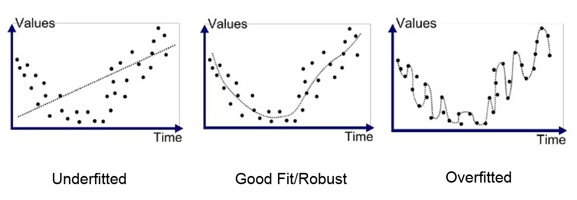
The problem with using linear regression in this way is that as the order of complexity increases, some of the proxy currencies may become overemphasized, and over-fitting becomes a real risk. Linear regression is also overly sensitive to noisy data. Figure 4 illustrates the concept of over-fitting, in which the algorithm tries to fit every nuance in the data (some of which is just noise) and in doing will perform poorly with data outside the original set. A lower-order fit (as in the middle diagram) is closer to the optimum model.
Figure 4
The Challenge with Linear Regression Is Finding the Right Level of Sensitivity
The good news is that new machine learning libraries include regression algorithms that can overcome the over-fitting tendencies of classical linear regression. Two common algorithms are:
- Ridge regression, which performs what is known as “regularization adding a penalty to the square of the magnitude of the weights. The penalty is a coefficient α times the sum of the squares of the weights. As α increases, the model complexity falls.
- Bayesian regression uses probability distributions rather than point estimates. Ŷ is not estimated as a vector of single values; instead, it is assumed to be drawn from a probability distribution. The aim of Bayesian linear regression is not to find the single, best value for each of the model’s parameters, but rather to determine the posterior distribution for the model’s parameters. Not only is the response generated from a probability distribution, but the model’s inputs are assumed to come from a distribution as well.
How to Implement Ridge or Bayesian Regression Analysis
To minimize basis risk, an FX risk manager must adopt the most robust approach possible for identifying effective currency proxies. I recommend starting with five years’ worth of monthly spot prices for all currencies you are considering including in the basket. (Historical spot FX rates are available at openfxrates.org.) I like a monthly cadence because more frequently collected data is too noisy, and hedging is generally on a monthly or longer scale. Five years gives plenty of history without including macroeconomic events that are no longer relevant. In fact, in my analyses, I’ve found that including 10 years’ worth of prices actually provides less-accurate fitting than five years.
Once you have your data set, machine learning algorithms found in Python Scipy or R libraries include several innovative techniques for making the most of the available data. The first technique is to split the data into two sets: one for training the algorithm and one for testing its results. The training set is used to build the model (i.e., identify weights for proxy currencies). Then the test set is used to measure how well the solution is generalized, as the model hasn’t “seen” the test data.
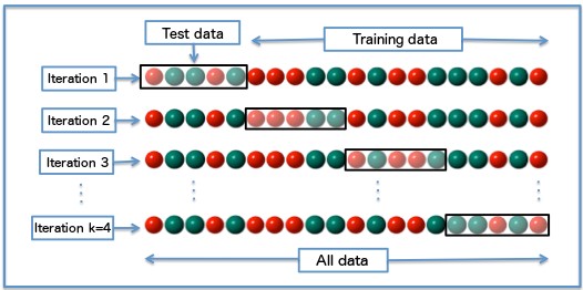
The second technique is called k-fold cross-validation. It selects the training and testing sets from multiple regularly partitioned “folds” of the data. This results in test data being drawn from all parts of the dataset. See Figure 5.
Figure 5
Drawing Test Data from k Number of Folds
My testing indicates that the machine learning approach works very well for numerous emerging-market currencies. Figure 5 shows the results of using machine learning to develop a basket that properly weights NZD, CAD, and AUD to serve as proxies for a USD-CLP exposure. I ran the Ridge regression algorithm to determine the appropriate weight of each currency in the basket, then calculated the actual results of the basket over a 60-month time frame.
The vertical axis in Figure 5 represents the price of the CLP vs. USD (i.e., Y). The horizontal axis shows the weighted value of my proxy-currency basket vs. USD (i.e., Ŷ). The line in Figure 5 represents an ideal hedge, the intersection at which the value of the proxy basket is identical to the price of the CLP. The scatter plot in Figure 6 illustrates the actual performance of my hypothetical hedge: correlation between the proxy basket and the actual price of the CLP, with one dot for each of the 60 month-ends.
Figure 6
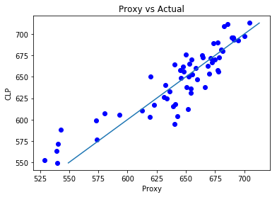
The results are strong—the correlation (i.e., R2) between the synthetic NDF and the target asset is 0.91. The mean error across all the data points is 0.6 percent, with a standard deviation of 3.4 percent.
To review the process: The data was processed using either Ridge or Bayeisan Regression, which identified the most effective weight (wj) for each of my M number of proxies. The software then used these M weights to calculate the Ŷ (proxy value) for each of the 60 rows in the array X. In Figure 5, the Ŷ values are plotted along the horizontal axis; the corresponding value of the currency to which I have an exposure (Y), for each date, is plotted along the vertical axis. The mean error and standard deviation are measured across all 60 rows, meaning the level of accuracy holds across five years’ worth of data.
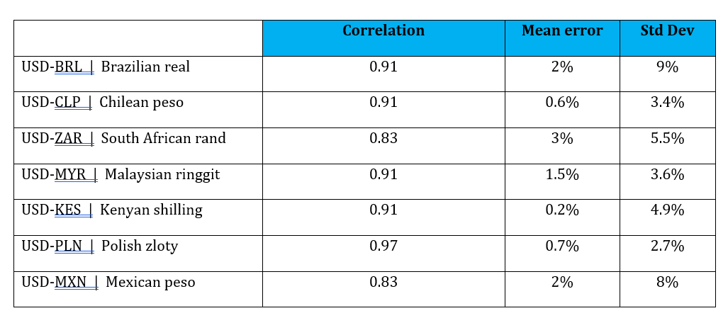
I have tested specific proxies for many different emerging-market currencies with this approach, using both Ridge and Bayesian regression. Figure 6 shows some highlights of that testing.
Figure 7
Effectiveness of Hedging Baskets of Various Proxy Currencies
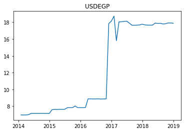
Some currencies do not lend themselves to this approach. For example, the BDT (Bangladeshi taka), TWD (Taiwanese dollar), and XOF (West African CFA franc) proved immune to this approach. Such a mismatch is generally the result of the currency moving relative to the USD in ways so irregular that no set of proxies can match them. Other currencies that have been affected by recent and extreme historical events, such as the EGP (Egyptian pound) are equally difficult; see Figure 8.
Figure 8
USD/ EGP over Five Years
Finding the Optimum Hedge Ratio
When there is basis risk, the optimum hedge ratio will minimize variance between the combined hedge position and movement of our target asset[1]. With our machine learning NDF based on a basket of weighted proxies, we want to minimize:
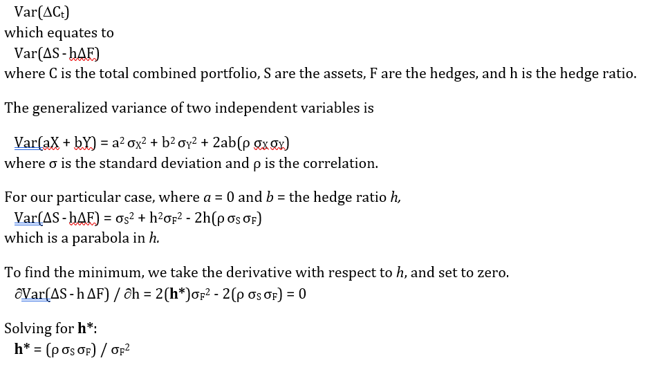
For our example in hedging CLP, the standard deviation of Y (predicted) is 61, and the standard deviation of the target is 55. This gives an optimum hedge ratio of 0.812. Then we can use this to calculate the actual hedge notionals. In our example, the firm’s exposure to CLP is equivalent to $1 million of USD.
Using the optimum hedge ratio and the coefficients (weights) determined by Ridge regression, the proxy hedge amounts are:
- buy $279,752 USD, sell NZD
- buy $263,776 USD, sell AUD
- buy $268,916 USD, sell CAD
for a total of $812,444 in USD.
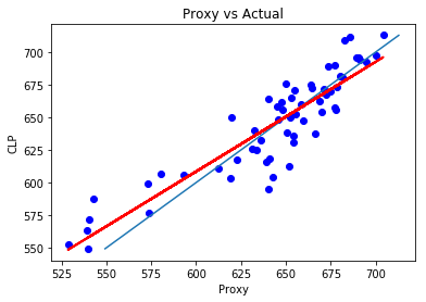
If we fit a line to the synthetic NDF (the red line in Figure 9), we see that it has a slightly shallower slope than the “perfect” fit from Figure 5. The red line illustrates the optimum hedge ratio. This makes sense intuitively, as the target asset’s volatility is slightly smaller than the volatility of the proxy currency basket, so the hedge should be slightly smaller than the $1 million exposure.
Figure 9
I have used this process with other base currencies in addition to USD, such as EUR and GBP. The process works identically. Sometimes, one base currency works better than others. For example, in my testing, USD works better than GBP when hedging Malagasy Ariary (MGA). In response, the proxy trades would be based on USD, with one more trade to transfer the results from GBP to USD.
Experimentation with proxy currencies is worthwhile. Sometimes using three proxies works as well as four. Occasionally, the Bayesian regression finds the closest correlation if the basket consists of three trades in one direction and a fourth currency traded in the other direction. Such an approach is generally undesirable, though. The combination of hedges might make the proxy more accurate, but the increase in traded notionals is generally undesirable. I would tend to recommend dropping the opposite-direction proxy and re-determining the weights of the other currencies in the basket.
Conclusions
When the markets are smoothly functioning, the likelihood of errors is minimal and basis risk is low for many emerging market currencies. But what happens when markets are disrupted, like they were in 2008? Correlations among currencies may not continue to follow historical trends, as each economy will react differently.
Using data from the period of 2007–2012, we found that the mean error in currency correlations was very similar during that period to what our model would lead us to expect, but the standard deviations increased materially, generally by about 50 percent. For the treasurer looking to mitigate FX risk, this would have the effect of reducing the optimum hedge ratio.
All in all, proxy hedging is a useful strategy for mitigating risk around currencies for which hedging instruments are unavailable, illiquid, or prohibitively expensive. The challenge has always been identifying the best proxy currency. Treasurers can solve this problem by creating a synthetic NDF using three to four major currencies whose liquidity is high and whose cost is low. Applying machine learning algorithms that incorporate regularization sidesteps the potential instability and over-fitting of an ordinary linear regression.
The results are very usable for many emerging-market currencies: The correlation between the asset and synthetic proxy is high (85 to 95 percent) and prediction errors are very low (average error of 2 to 3 percent). This makes the hedging of African, Asian, and South American currencies both practical and affordable.
Of course, a proxy hedge offers no ironclad guarantee of efficacy; hedging always entails a basis risk. However, when a treasurer’s only option is to use a proxy hedge, spreading that proxy function among multiple currencies can vastly reduce the chance that a macro event in one economy will destroy the correlation altogether.
Paul Stafford is managing director of Currency Risk Management, LLC. He graduated from the University of California, Berkeley with a bachelor’s degree in engineering and continued engineering studies at Stanford University. After working at NASA and Hewlett-Packard, Stafford turned his analytics abilities to the foreign exchange markets and derivatives.
[1] Hull, Options, Futures and other Derivatives (8th ed.)
Reprinted with permission from the October 10, 2019, online edition of Treasury & Risk © 2019 ALM Media Properties, LLC. All rights reserved. Further duplication without permission is prohibited, contact 877-257-3382 or reprints@alm.com.