While the Treasury dept is not R&D, there is a surprising amount of mathematics involved. From yield spread analysis, term structure of interest rates, zero-coupon yield curve, price/yield analysis and other concepts; the Treasurer or CFO is required to know more than a little mathematics. While bond and interest rate issues constitute the lions share, the foreign exchange component also requires maths- covered interest rate parity, forward point rate curves, value at risk and option valuation are just a few of the more complex concepts. This paper will provide an overview of the more common maths required in managing FX risk in the corporate context. We will start off gently, and work up to more complex ideas.
Spot conversion logic (cancelation of units)
Starting off with arithmetic lets address conversion of currencies. Let's begin with a review of what the spot rate means. It is the ratio of the base currency to the term currency:
Base/Term = spot. For example, GBP/USD = 1.3164, or USD/GBP = .7481
The base currency can be either the foreign (local) ccy, and the term/functional ccy, or the reverse, depending upon convenience and convention. There is an ISO standard that recommends certain conventions, but not even bank blotters strictly adhere to it.
If we have GBP/USD and EUR/USD, we have what we need to obtain GBPEUR. But if we simply multiply those two numbers together (1.3164 * 1.1562), we would get the wrong answer. To ensure the correct result, recall your high school physics and unit cancellation. We need to invert the EUR/USD to USD/EUR so the USD will cancel.

Now we have 1.3164 * .8649 = 1.1386, which is the correct spot for GBPEUR.
Forward point calculation
With that gentle arithmetic introduction, let's move on to the forward rate. The forward exchange rate is the rate at which a counterparty agrees to exchange a notional amount of currency for another at a future date. This agreement is often used as a risk management tool, ensuring a known rate for future payables or receivables. The forward rate cannot be the same as the spot rate at inception because otherwise, the differential deposit rate between the two countries would create an opportunity for riskless arbitrage (the arbitrageur would borrow currency with the lower rate, convert at today's spot rate, and invest in the foreign currency with the higher rate, converting back at the original spot rate). The forward rate is determined by three variables- the present spot rate, the domestic interest rate, and the foreign interest rate. The equation which sets the no-arbitrage condition is easy to derive. The rate of return for the foreign funds must equal the rate on domestic funds when converted at the future-forward rate:
(1+ if) = S*(1+id)÷F
eq 1
Where F is the forward rate, S is the spot rate, id is the domestic interest rate, and if is the foreign interest rate.
If we solve for the forward rate by multiplying both sides by F and dividing both sides by (1+if), we get:
F = S*(1+id)/ (1+ if)
eq 2
Interest rates will vary depending upon tenor, so the forward rate for a one month forward will be quite different than one for 6 months. Here is a worked example. The current EURGBP spot rate = .8785, the domestic one month rate is .1%, and the foreign rate is .15%. A moment with a calculator or Excel™ reveals the forward rate to be .8788. Note that the forward rate may be less than or greater than the spot rate. This means that FX hedgers may either profit by; or pay to lock in future rates. For emerging market currencies with high domestic interest rates, forward rates may be quite material.
Optimum tenor
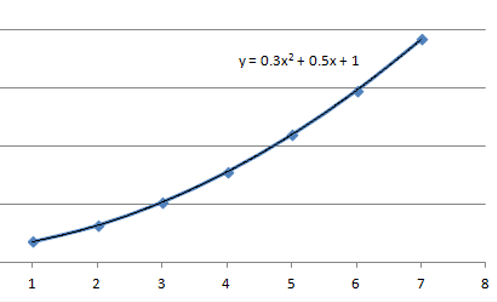
One common determination Treasurers/CFOs make is the optimum tenor of a hedge. For longer tenors, they can either enter into a single long-tenor contract or roll multiple shorter tenors. Determining the curvature of the yield curve will help in optimizing the tenor. If the line is linear, there is no advantage to longer tenors. If the curvature is upwards, it's best to roll shorter tenors than select longer ones, and if the curvature is negative, longer tenors are the best choice. One easy way to calculate the curvature (if it's not visually apparent) is to put the tenors and yields into Excel and plot the data. Clicking on the plotted data line, select "add trend line" and "display equation on chart". If the second-order coefficient is positive (as in the fig below, + 0.3), the curvature is also positive, and it's best to use shorter tenors.
Normal distribution
Normal distributions are often used in finance to represent random variables whose distributions aren't known a priori. It is also referred to as the "bell curve" (inaccurately - many other distributions such as Cauchy or Student's-t are similarly-shaped. According to Wikipedia, "The normal distribution is useful because of the central limit theorem. In its most general form, under some conditions (which include finite variance), it states that averages of samples of observations of random variables independently drawn from independent distributions converge in distribution to the normal, that is, become normally distributed when the number of observations is sufficiently large."[1]
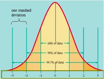
There are two main variables that describe the shape. The mean, µ ("mu") describes the mean or expectation of the distribution. Its value in the standard normal distribution is 0. The standard deviation, σ ("sigma"), describes the dispersion of the data about the mean. A low σ means that the data points will cluster close to the mean, and a high σ means the data will be more spread out.
So where is the normal distribution used in finance and Treasury? The main use is in the modeling of the market, pricing of options, and measurement of risk. Price movements are assumed to be normally distributed. This is a matter of practicality, not science, as any observer of the markets can tell you! Black Swans, Central Bank shocks and other real-world events disrupt smooth, tractable models. The real world is complex, but unfortunately most ‘complex’ distributions do not have a defining equation. Having an equation for a distribution means the distribution is ‘closed-form’, which makes it practical to calculate probabilities, confidence intervals, & manipulate using Excel for tasks such as doing Monte Carlo simulations. The equation describing a normal distribution is:
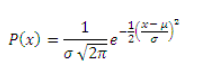
You do not have to use this equation directly (unless you really want to) - Excel has a number of built-in statistical functions such as NORMSINV, NORMDIST to handle the underlying complexity.
There is one more important distribution, the "lognormal" distribution. It is normally used to model asset prices whose returns are normally distributed. The reason for its use is that a series of lognormal returns are additive. For example, if you took a series of stock returns and measured their return in percent, you could not take the sum of the percents, multiply by the first price, and arrive at the end price. However, taking the log of the returns is additive. Again, Excel saves the day with the LOGNORMDDIST function.
One practical application of the normal is determining the (historical) volatility of a currency pair. Since the standard deviation σ measures dispersion, it is used as a proxy for volatility. Using Excel and any number of online spot history services (e.g. OFX[2]), create a column of daily series of price history. Before calculating the volatility, these spot prices must be converted to log-normal returns. Make a new column where the value = ln(N/N-1). Use the STDDEV Excel function on this new column to obtain the daily volatility. To convert to other periods (eg quarterly, annual, etc), the square root rule comes into play. Volatility is proportional to the square root of time, so it's easy to convert from one to the other. But why does it work?
We assumed that prices follow a random walk, (a.k.a. Brownian Motion). Each particular increment of this random walk has a variance that is proportional to the time over which the price was moving. For example, if a particular randomly moving stock has variance equal to 1 in 1 day, it has variance equal to 2 in 2 days, etc. Volatility or standard deviation is the square root of variance.
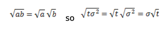
For example, let's say you found that the daily volatility of the EURUSD was .8%. To convert to annual volatility (say to calculate the Value at Risk, which we'll address shortly), we multiply the square root of the number of trading days, √ (252) * .8% = 12.7%
Value at risk
Building on our understanding of normal distributions as a model of price variation, we turn to Value at Risk, or VaR. VaR is commonly used to measure the risk in a portfolio (such as foreign currency-denominated assets or liabilities). If we review the normal distribution model again:

We see that 68% of data fall within +/- one σ, 95% falls within +/- two σ, etc. We can use this to model a level of confidence that price movements will remain within a range with certain percent confidence. Industry practice is to select a standard confidence interval (90%, 95%, 99%). These "confidence intervals" drive the calculation of the "Z value", which is simply the number of standard deviations. 90% corresponds to 1.28 σ , 95% to 1.644 σ , and 99% to 2.32 σ [3]. Now it becomes a simple matter to calculate the annual VaR of an exposure. Our hypothetical exposure = €1M. The historical daily volatility is .75%, and we select a confidence interval of 95%. VaR = €1M * 1.644*.75%*√ (252) = €199k. We interpret this as the maximum expected loss in a year, with a 95% confidence.
Review
- · Spot quotes - Pay careful note to which currency is base, and which is term. Find daily and historical values at https://www.ofx.com/en-us/forex-news/historical-exchange-rates/
- Forward rates - You don't need to start with interest rates - find current forward points at https://uk.investing.com/rates-bonds/forward-rates. Note that they are quoted here in basis points and need to be divided by 10,000 to add to the spot rate.
- Long-tenor hedges may be hedged with either long tenors or short tenors which are rolled periodically. The forward curve shows which are most advantageous.
- Volatility - Assuming a normal distribution simplifies many calculations. However, models have their limitations! the real world is not so neat and includes surprises.
- Value-at-Risk is an important first step in quantifying risk and planning on how to manage it.
A Treasurers or CFO who is familiar with the mathematics of FX will be more effective, independent and able to translate or explain these concepts to C-suite mgmt, or shareholders.
[1] https://en.wikipedia.org/wiki/Normal_distribution
[2] https://www.ofx.com/en-us/forex-news/historical-exchange-rates/
[3] if you desire another confidence interval, Excel's NORMSINV function will calculate the Z value.
Deaglo work with Investment Managers, Investors and Companies to better execute and mitigate risk with FX transactions. Reach out to one of our team now.