Often, investment portfolios are exposed to multiple currencies. For those that choose to hedge all or part of this exposure, determining the optimal hedge strategy is a difficult task. Each exposure has different individual characteristics: notional size, volatility, and cost of hedging. Additionally, many currency pairs are positively or negatively correlated. The potential is high for under or over-hedging risk or spending too much to manage it altogether. The impact of oversimplifying the task (e.g. passively-selecting a fixed hedge ratio across the portfolio) is either excess risk, excess hedge costs, or both.
Example portfolio
Let's pose a hypothetical USD-based fund which is long 5 different currencies; CAD, GBP, EUR, BRL and MXN; a mix of developed country and EM investments. Table 1 describes the size of the exposure (notional), the cost of hedging (1-month fwd rates), and two measures of risk- the volatilities, and the correlations between the currencies.

It's not clear at all what the hedging priorities should be! CAD is the largest exposure but has the lowest volatility, and a small negative hedge cost. MXN and BRL are more complicated- they have lower notionals, but high volatility and high cost of hedging. With 5 different ccy pairs, all of which have different characteristics; it's impossible to judge empirically what hedge ratio should be adopted for each. Moreover, the practitioner has a difficult time quantifying portfolio-level risk, as some of the exposures are negatively correlated with others (in other words, there is some level of natural hedging). Simply adopting a constant hedge ratio across the portfolio will not achieve an optimum ratio of risk reduction per unit hedge cost. A more robust mathematical approach for determining optimum hedge ratio for each portfolio element is warranted.
Two challenges
The first challenge is to calculate a representation of portfolio-wide risk which incorporates all four factors (size, cost, volatility, covariance) simultaneously. We start with the daily excess returns (log return - mean) of each currency pair over the most recent year. Using this array, we calculate the variance-covariance matrix.
The resulting matrix gives us both the variance of each currency (the square of the standard deviation, aka volatility), and the covariance (a measure of how correlated each currency pair is with the other). We represent a potential hedge ratio solution - the Risk Vector - with a matrix consisting of the unhedged notional fraction. We project the Risk vector onto the VarCovar matrix, which will result in a scalar representation of portfolio variance.
The second challenge is to find the optimum combination of hedge ratios to minimize the hedge cost per unit portfolio variance. This requires optimizing 5 variables (hedge ratio for each currency pair) simultaneously. We could use brute force, but that would require prodigious computational time (and the inelegance offends!). Instead, we turn to Convex Optimization. The standard form for convex optimization consists of three parts:
minimize f(x)
subject to: gi(x) ≤ 0, i = 1,.., m
hi(x) = 0, i = 1,...,p where h has to be affine
In our case, h(x) is the cost function, which is simply the exposure notional * hedge ratio * fwd points. g(x) is our portfolio variance calculation as described above. As the variance is allowed to range from zero to the max VaR, the optimizer determines the hedge ratios for each of the currency pairs. This results in the identification of an "efficiency frontier" (EF, fig 1). Each point on the line represents a hedge ratio for each portfolio member.
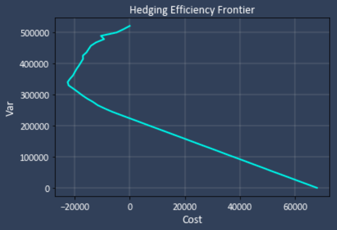
This particular frontier (representing the exposures in table 1) is interesting. The upper endpoint (zero cost, max VaR) represents no hedging at all. The bottom right point represents full hedging- zero VaR, max cost). The first section shows how VaR drops off slowly, but with profitable hedge points, then crossing into more costly hedging as VaR is further reduced. Once the EF line is determined, the practitioner simply chooses a point along the line, prioritizing either cost or risk as desired. The selected point corresponds to a set of the correct hedge ratio for each element in the portfolio to achieve the EF point. At one point, the cost is zero, and the one month VaR95% has dropped from 520,000 to 223,000.
It's important to recognize that the efficiency frontier represents the best possible combination of hedge ratios - for any given level of VaR, there is no lower cost possible.
This works very well for the corporate CFO hedging his assets and liabilities (both forecast or realized). It also works for the FX passive overlay manager of an investment or pension fund, managing NAV spread across multiple countries and currencies. The savings can be large.
Here's another example. The exposures are a combination of majors and multiple EM currencies.
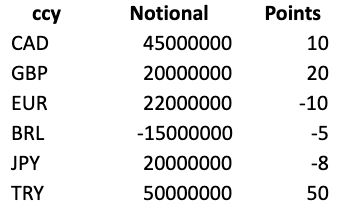
There is some correlation between BRL and TRY. The hedge frontier is now:

An interesting characteristic of this approach is that FX exposures represent generic risk exposures. the names of the currency pairs (USDBRL, etc) are simply names. Other asset classes can be optimized along with FX. Many corporates hold excess cash in bonds, and funds often invest in bonds. The value of those bonds varies as the yield curve changes market expectations of return. This creates interest rate risk. Additionally, corporates are often exposed to commodity risk. In its purest form, this is the variation in the cost of raw materials (iron, aluminum, etc). It can also be the cost of energy (directly or indirectly), or transportation costs (eg RBOB or Gasoil futures).
The EF risk management concept can manage all of these risks, even across asset class lines. The reason it can do so is simple- each of those assets has the same characteristics as the assets in the FX class alone - a notional size, a cost to hedge, volatility, and a correlation with the other assets. The benefits to the corporate are an increase in the cost-benefit of hedging, and an increase in their Sharpe Ratio (reduction in beta).
Operational considerations
- The assets must all hedged with the same tenor (eg 3 months, 6 months).
- For a fund that is often rebalancing its portfolio, the optimization should be run as often as necessary. A recalculation of the VarCovar matrix may indicate a material variance from the prior period (perhaps due to some macro event). It is then prudent to recalculate and readjust hedge ratios.
- If non-linear hedging derivatives are used (e.g. options and exotics like barriers, knock-ins/outs, or look-backs), convex optimization cannot be used (the solution space is no longer an affine set), and a Monte Carlo simulation should be used instead.
- For investment funds with foreign bonds, often the fund is looking for exposure to a part of the IR risk (eg they may have a steepener on). In this case, it is a simple matter to hedge only the components they do not want exposure to (correspondingly, level and curvature).
Conclusion
For firms and funds with FX, commodity risk or IR risk, managing them separately and in fixed hedge ratios is inefficient and costly. The use of Risk Vectors and VarCovar matrices to determine scalar portfolio risk; and optimization techniques to determine an efficient hedging frontier from which the optimum hedging solution may be selected is a robust and efficient solution.