Funds are exposed to currency effects from non-base currency investments in their portfolio. Those effects may be intentional (currency treated as an "asset" class), but this is often not the case and therefore, becomes FX risk. This FX risk can be managed with either a passive strategy or an active or dynamic strategy.
The passive approach seeks to simply negate the effects of currency on the value of the portfolio as measured in its base or home currency. This is generally accomplished using forward contracts or more often, swaps. The passive overlay manager's main challenge is to maximize hedge efficiency, within the constraints of the fund operations (frequency of valuation and rebalancing, cash flows and benchmarks).
An active or dynamic manager, on the other hand, treats currency effects as an asset class. For additional fees, the active overlay manager utilizes predictive models (which include macro-economic, market sentiment, technical analysis and other factors) to determine a hedge ratio that will not only protect the other asset classes but in some cases, actually generate alpha.
The pacifist's challenge
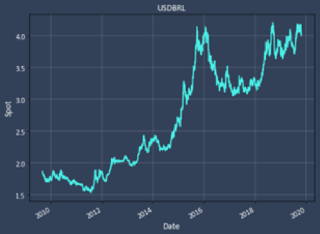
This article focuses on the passive overlay manager's task. Given the diversity of cross-border investments, often in liquidity-challenged emerging markets, the task is still challenging. Each asset/currency has its own, varying notional size, inherent volatility and hedge cost. Additionally, many of the currencies will exhibit some correlation with others in the portfolio. Those with negative correlations with each other will form a partial natural hedge. Thus, simply managing each portfolio exposure independently will result in over-hedging and excess hedge costs, reducing returns. Lastly, managing separate share classes adds an additional level of complexity. Without a proper fund and share class netting algorithm, double-hedging becomes almost a surety, further eroding returns.
Executing a passive overlay then becomes a two-step process.
- Determine the fund exposures as measured against the base currency. Calculate share class ownership fractions, and net the resulting two sets of exposures to arrive at a net fund exposure.
- Calculate the hedge ratios required to manage portfolio Value at Risk (VaR) to the desired level, accounting for portfolio member size, hedge cost and cross-correlation. Minimize hedge costs per unit VaR reduction.
The first task is straightforward arithmetic. The second, however, requires some clever maths. A most useful concept is the efficiency frontier, and in this context will represent the set of hedging solutions that minimizes portfolio VaR for any level of hedge cost. The overlay manager can then select the level of either hedge cost or VaR according to his performance metrics, and that point on the frontier yields the optimum hedge ratios for each portfolio member.
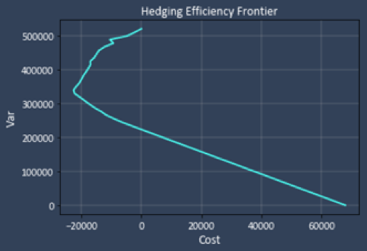
Fig 2 is an example of a hedging efficiency frontier. Portfolio VaR is on the y-axis, and hedge costs along the x-axis. As can be seen in this example, some of the forward points are in the hedger's favor, and the first 50% or so of VaR reduction is profitable or free. The overlay manager can select his preferred level of cost or VaR accordingly. The second step of the process is complete.
But how do we obtain this efficiency frontier? There are several key concepts and methods used to arrive at this highly-efficient passive overlay hedging process.
Under the hood/bonnet
We must have an algorithm for calculating the portfolio-level VaR. This single, scalar value must represent all of the portfolio element variability (size, cost, volatility and correlation). Alas, the portfolio VaR is not simply the arithmetic sum of the individual element VaRs, because of the correlations between them. We must start with the variance/covariance matrix (calculated from log returns), which is a matrix of both the volatility within each asset and the correlation between assets.
We then form a "Risk vector", consisting of the unhedged notional for each element. If we "project" this (n x 1) risk vector onto the (n x n) VarCovar matrix, we end up with the portfolio VaR scalar.
The last computational trick up our sleeves is to utilize constrained optimization, which will be used to generate the minimum VaR for each level of hedge cost.

We know the maximum portfolio VaR (nothing is hedged). By stepping from zero to the maximum VaR, at every point minimizing the hedge cost by optimizing hedge ratios within the portfolio, the efficiency frontier is generated.
While the passive overlay manager's job is easier than the active manager's there are still complexities to be overcome to achieve the most cost-efficient overlay plan. We have laid out a two-step process and described at a high level the computational tasks required to achieve the lowest cost per unit VaR reduction possible.
The team at Deaglo Partners has created a suite of services designed to alleviate the concerns when investing overseas. We represent both foreign investors and globally focused managers across all investment types and are always happy to jump on a call.